The
APCD model = Age Period Cohort – Detrended
Louis Chauvel
Site : www.louischauvel.org/apcdex
email : chauvel@louischauvel.org
This web page intends to present the STATA “ssc install apcd” ado file, its
methodological background and some examples.
1. Problems:
The problem with APC
models is the general lack of stability of linear trends of the age, period and
cohort estimates where appropriate constraints should be added in order to
obtain stable estimates, but there are still debates on this choice of
coefficients. In their APC_IE methodology, Yang and al. propose that a
Principal Component Analysis solve this problem, but the usefulness of this
choice is still debated (O’Brien 2011).
The “detrended cohort estimates” DCE estimates (see 2. Methods) proposes
a separation between linear trend analysis (that definitively can not be disentangled between age, period and cohort linear
effects) and fluctuations. This model is able to tackle better the trends
problem that other models generate, for example with education where the APC-IE
proposes a steady decline of educational level with age; in reality, the linear
trends of APC coefficients are generally not interpretable (see part 5 below).
2. Methods:
Please download the pdf: www.louischauvel.org/apcdmethodo.pdf where the main concepts are presented with
the model itself.
3. First
example: a cohort based variable: veterans
See the do file:
www.louischauvel.org/apcdvet.do
[here is an extract of the Ipums
US census and ACS 1980-2010, Steven Ruggles, J. Trent
Alexander, Katie Genadek, Ronald Goeken,
Matthew B. Schroeder, and Matthew Sobek. Integrated
Public Use Microdata Series: Version 5.0
[Machine-readable database].
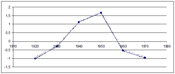
The status of veteran is deeply connected to birth cohorts. About 45% of
the male population born in 1947 was drafted for the Vietnam War while less
than 10% of those born before 1940 or after 1955 were. Wars are deep contexts
of cohort effect formation and it is why APC analysis of veterans make sense, but
more as a test of a cohort method than as a plan to make new discoveries.
The first step here is to test the apcd model
on Vietnam war veterans (viet=0/1)
in a logit APC-D model.
The contextual variables give significant elements, first for gender (!)
then for ethnicities: drop outs, Hispanics, other races (that are social groups
specific of a more or less recent entry in the
*******************************************
####### APC Detrended model #######
*******************************************
(623178 missing values
generated)
Iteration 0: log pseudolikelihood
= -1.303e+08
Iteration 1: log pseudolikelihood
= -1.060e+08
Iteration 2: log pseudolikelihood
= -1.051e+08
Iteration 3: log pseudolikelihood
= -1.051e+08
Iteration 4: log pseudolikelihood
= -1.051e+08
Generalized linear
models No. of obs = 571855
Optimization : ML Residual df =
571833
Scale parameter = 1
Deviance =
210179661.9 (1/df) Deviance = 367.5543
Pearson =
1071985128 (1/df) Pearson =
1874.647
Variance function: V(u) = u*(1-u) [Bernoulli]
Link function : g(u) = ln(u/(1-u))
[Logit]
AIC = 367.5402
Log pseudolikelihood
= -105089830.9 BIC = 2.03e+08
( 1) [viet]coh_1920 + [viet]coh_1930 + [viet]coh_1940 +
[viet]coh_1950 + [viet]coh_1960
+ [viet]coh_1970 = 0
( 2) - 5*[viet]coh_1920
- 3*[viet]coh_1930 - [viet]coh_1940
+ [viet]coh_1950 + 3*[viet]coh_1960
+ 5*[viet]coh_1970 = 0
( 3) [viet]age_0030 + [viet]age_0040 + [viet]age_0050 +
[viet]age_0060 + [viet]age_0070
= 0
( 4) - 4*[viet]age_0030
- 2*[viet]age_0040 + 2*[viet]age_0060
+ 4*[viet]age_0070 = 0
( 5) [viet]per_1980 + [viet]per_1990 + [viet]per_2000 +
[viet]per_2010 = 0
( 6) - 3*[viet]per_1980
- [viet]per_1990 + [viet]per_2000
+ 3*[viet]per_2010 = 0
------------------------------------------------------------------------------
| Robust
viet
| Coef. Std. Err. z P>|z|
[95% Conf. Interval]
-------------+----------------------------------------------------------------
coh_1920 | -.9707834 .0232047
-41.84 0.000 -1.016264
-.925303
coh_1930 | -.3195585 .0235933
-13.54 0.000 -.3658006
-.2733165
coh_1940 |
1.115685 .015823 70.51
0.000 1.084672 1.146697
coh_1950 |
1.658306 .0150098 110.48
0.000 1.628887 1.687725
coh_1960 | -.5315142 .0242539
-21.91 0.000 -.5790511
-.4839773
coh_1970 | -.9521343 .0243227
-39.15 0.000 -.9998058
-.9044627
age_0030 |
.0117883 .0099741 1.18
0.237 -.0077605 .0313371
age_0040 | -.0218496 .0118446
-1.84 0.065 -.0450646
.0013655
age_0050 | .024114
.0131639 1.83 0.067
-.0016867 .0499147
age_0060 | -.0298326 .0131493
-2.27 0.023 -.0556049
-.0040604
age_0070 |
.0157799 .0109327 1.44
0.149 -.0056478 .0372076
per_1980 |
.0050198 .0076948 0.65
0.514 -.0100618 .0201014
per_1990 | -.0105417 .0112558
-0.94 0.349 -.0326027
.0115193
per_2000 |
.0060241 .0115525 0.52
0.602 -.0166184 .0286666
per_2010 | -.0005021 .00784
-0.06 0.949 -.0158683 .014864
rescacoh
| -.6195064 .0392983
-15.76 0.000 -.6965297
-.542483
rescaage
| .0197929 .0126496
1.56 0.118 -.0049998
.0445856
hispan
| -.3166048 .0304606
-10.39 0.000 -.3763066
-.2569031
aa
| -.0960236 .0226548
-4.24 0.000 -.1404262
-.051621
sex | -2.464644
.0198651 -124.07 0.000
-2.503579 -2.425709
orace
| -.4056752 .0317338
-12.78 0.000 -.4678723
-.343478
_Ieduc_5 |
.4058921 .048345 8.40
0.000 .3111377 .5006465
_Ieduc_6 |
.8972972 .0272275 32.96
0.000 .8439322 .9506621
_Ieduc_7 |
1.130047 .0298255 37.89
0.000 1.07159 1.188504
_Ieduc_8 |
1.200131 .0318622 37.67
0.000 1.137682 1.26258
_Ieduc_9 | .722688
.030655 23.57 0.000
.6626053 .7827706
_Ieduc_10 |
.6184479 .0318983 19.39
0.000 .5559285
.6809674
_cons | -.8965447 .0319209
-28.09 0.000 -.9591085
-.8339808
------------------------------------------------------------------------------
(36 missing values
generated)
(36 missing values
generated)
*******************************************
Delta Bic
= -27506167
*******************************************
Figure3.1: shape
of cohort coefficients of Vietnam veterans
4. second example:
education
Education is, in the
set of common variables, one of the most influenced by birth cohort. The period
of entry in the age of choice between following education or
finding one’s independent life is strategic, in terms of opportunities or
limits.
www.louischauvel.org/apcdcpseduc.do
[here is an extract
of 1975-2010 (each 5 years) March CPS extracts source IPUMS, see: Miriam King,
Steven Ruggles, J. Trent Alexander, Sarah Flood,
Katie Genadek, Matthew B. Schroeder, Brandon Trampe, and Rebecca Vick. Integrated Public Use Microdata Series, Current Population Survey: Version 3.0. [Machine-readable database].
Figure4.1: % of BA degree owners (or higher) at
age 45 by birth cohort
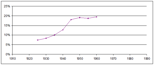
These data show the
extreme acceleration in educational resources of the cohorts born in early baby
boom (circa 1950). David Card (xxxx) and Robert Mare
(xxxx) have documented this singularity; the first
one insist in the Vietnam war context that increased
the incentive to follow education, and the second one on the composition
effects of immigration.
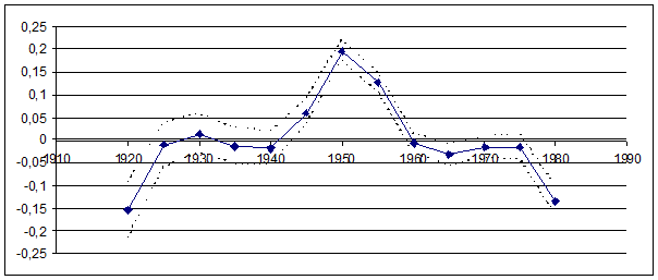
When we control by
usual contextual variables, the APCD model shows the specificity of the early
baby boom. These specific traits has been largely commented (xxx)
Figure4.2: shape of cohort coefficients of BA
degree owners (or higher) in the USA
The intensity of the cohort fluctuations for MA
owners is even stronger, and it is amazing that these gaps have received so
modest interest in the sociological literature. For MA owners, a part of the
gap is absorbed over life course (H=-.16), that is significant. This trend of
slight hysteresis could be due to the fact that cohorts with lower achievements
in terms of Ma degree can (partially) catch up later.
Figure4.3: % of MA degree owners (or higher) at
age 30, 40 & 50 by birth cohort
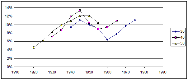
Figure8: shape of cohort coefficients of MA
degree owners (or higher) in the
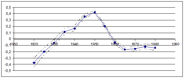
This means that birth cohort is an important
parameter of inequality of distribution of education, since the context of
educational development between age 17 and 23 is of major importance for
individual’s opportunities. More precisely, the cohorts born in the late
1940’s, beginning of the 1950’s, have benefited from exceptional opportunities
for having longer education. A major aspect of Age-Period-Cohort specificities
in the
5. third example:
education and a comparison with Yang’s APC-IE
Here is an example of the limits of the Yang’s
and colleagues apc_ie
(intrinsic estimator) model. The aim of the ie is to
provide a “per se” optimal age, period and cohort trend. When we make use of
the apc_ie model for BA or higher owners, education
seams to increase with period and to decrease with age, which is sociologically
misleading.
www.louischauvel.org/apcdcpseduc.do
Figure5.1: shape of age, period and cohort
coefficients of BA degree owners (or higher) in the US, after the Yang’s apc_ie model
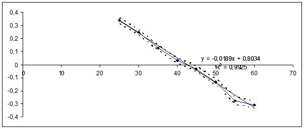
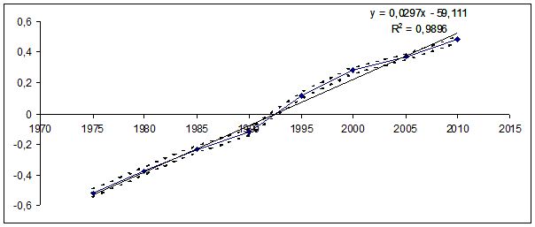
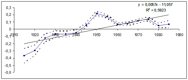
In the general case, the linear trends of the
age, period and cohort coefficient can not be interpreted easily and appear
more as technical intercepts than as meaningful results. It is why we must
prefer the detrended approach, where the real focus is driven to the shocks
below or above the linear trends.