Odds ratios erratic changes: a problematic
simulation
Louis Chauvel
To download the text in acrobat click here
Intentions
The
technology based on odd ratios is supposed to solve the problem of
comparability of statistical links in tables where the marginal structures
change. For the last 25 years, major advances in intergenerational mobility
analyses have resulted from odds-ratio based statistical models.
My
intention is here to show a limit of the use of odds ratios that can raise some
doubts on different results: in a realistic example, we can notice significant
and substantial changes in the odds-ratios when the intrinsic statistical link
(in this example in terms of homogamy) remains unchanged. Then, some
methodological developments on the odds-ratio are required to know when the
odds ratio is an accurate measure of real evolutions and when it is not.
The
odds-ratio (if you know what it is, please skip to the next item)
I have
little space here for developments on the odds ratios. They are supposed to be
a measure statistical links between two variables which is robust when the
marginal distributions of variable changes. For example, the central problem of
the measure of the degree of social mobility in intergenerational tables is the
changes in the line and column margins for one period to another (relative
decline of workers, expansion of managers and experts, etc.). If fathers
(social origins) are in lines and sons (social destination) in columns, the
cross tables of two countries could give non evident results simply because the
social structures (the margins of the tables) differ. How to compare? The odds
ratio is an answer. On the first table of 6000 fathers and sons, the odds ratio
is the ratio of the product of diagonal cells (800x5000) by the product of
anti-diagonal cells (150x50), and the result is 533. On the second table, the
odds ratio is 147.
Example of mobility table
|
Country 1 |
|
|
|
|
|
|
father son |
worker |
white collar |
Marg.F |
|
|
|
worker |
5000 |
150 |
5150 |
|
|
|
white collar |
50 |
800 |
850 |
OR= |
533,3 |
|
Marg.S |
5050 |
950 |
6000 |
|
|
|
Country
2 |
|
|
|
|
|
|
father son |
worker |
white collar |
Marg.F |
|
|
|
worker |
4500 |
550 |
5050 |
|
|
|
white collar |
50 |
900 |
950 |
OR= |
147,3 |
|
Marg.S |
4550 |
1450 |
6000 |
|
|
When the
Odds ratio is 1, the origin (father occupation) and his son destination are
independent variables. An Odds ratio could have a value inferior to 1 if the
probability to become worker are higher for those with white collar origins than
for those with worker origins. The higher the odds ratio, the stronger the link
between origins and destinations. The country described in the second table is
supposed to more fluid (more mobile, more permeable) than the first one: the
impact of origin on destination is lower.
A
problematic example
The odds
ratio is an efficient tool with categorical data where social groups or social
classes are defied by clear frontiers. Anyway, we can face problems when the
implicit process pertains to numeric variables. It is often the context with
education where the (categorical) level of education depends on the (numeric)
duration of exposure to teaching. I present here an example where the
statistical link between the level of education of men and women in couples
remain unchanged, in a context of educational expansion, but when the
odds-ratios significantly decline.
Then,
consider the level of education of members of couples. Suppose the age at end
of education (maleendedu and femaendedu, a numeric variable) is the central
determination of the level of education (1 lower, 2 intermediate, 3 higher, a
categorical variable). The higher educational group (maledip=3 or femadip=3) is
defined by and endedu greater than age 23; the intermediate group of education
is for people between age 18 (included) and age 23 (excluded) (maledip=2). The
lower one is bellow age 18 (excluded) (maledip=1).
For men and
women in couples, we consider the distribution of endedu (age at end of
education) as a normal distribution with a standard deviation of 3,79. The
average endedu depends on generation. We have 5 generations (gen = -2, �C1, 0,
1, 2). The average endedu for the first generation is age 16, age 17 for the
second�� to age 20 for the fifth one.
Inside each
generation, the coefficient of linear correlation between the endedu of male
and the endedu of female is stable with an R2 of 0.385 (R=0.62). The
change from generation �C2 to generation 2 is simply a shift from average age 16
to average age 20 of the average of endedu for men and women (educational
expansion).
In this
example, an accurate measure of educational homogamy should provide a diagnosis
in terms of stability. But, here, the odds ratios pertaining to educational
levels (maledip and femadip from 1 to 3) show significant if not dramatic
changes.
Rules
and simulation
With the
rules given below, we simulate 250.000 random couples, on 5 generations of
50.000 couples, and the consequences of an educational expansion in terms of
homogamy are measured by the odds-ratio. The 250.000 lines table (tabulated
text of 5.8 MegaB) is provided in a separate file that can be freely downloaded
on this site http://louis.chauvel.free.fr/oddodds.dat .
A source
variable (randnorm) is a normal random variable (E = 0 and SD = 2).
The
variable gen indexes five generations (from �C2 to +2).
The
variables maleendedu and femaendedu are the ceiling of the sum of randnorm*1.5,
of a normal random variable (E = 0 and SD = 2.3), of 17.5 (the overall
average), and of variable gen (in 5 generations, the average of endedu
increases of 5 years). The formula for women is the same.
maleendedu
= Ceiling(Random Normal() * 2.3 +
randnorm * 1.5 + 17.5 + gen)
The level
of education (maledip and femadip) is a 3 modalities categorical variable. The
higher educational group (dip=3) is defined by an endedu greater than age 23;
the intermediate group (2) is between age 18 (included) and age 23 (excluded).
The lower group (1) is bellow age 18 (excluded).
Results
The table
of the results of the simulation on the 5 generations of 50.000 random couples
are given here : (the randomization has been launched several times, over 30,
and the results were ever similar).
The aggregate table (250.000 individuals)
|
|
|
gen |
|
|
|
|
|
maledip |
femadip |
-2 |
-1 |
0 |
1 |
2 |
|
1 |
1 |
26117 |
20776 |
15363 |
10762 |
6946 |
|
1 |
2 |
6229 |
6682 |
6682 |
6119 |
5007 |
|
1 |
3 |
243 |
326 |
464 |
501 |
539 |
|
2 |
1 |
6310 |
6735 |
6542 |
6190 |
5127 |
|
2 |
2 |
7682 |
9981 |
12240 |
13721 |
14450 |
|
2 |
3 |
1224 |
2019 |
2896 |
3907 |
5179 |
|
3 |
1 |
255 |
363 |
415 |
477 |
504 |
|
3 |
2 |
1239 |
1819 |
2939 |
3979 |
5111 |
|
3 |
3 |
701 |
1299 |
2459 |
4344 |
7137 |
We can calculate
the LOR, log odds ratios of tables of maledip and femadip 1x2, 2x3 and 1x3, for
the five generations. For instance:
We compute
the different LOR and their 95% confidence intervals (Agresti, 1984): the
standard error of LOR is the square root of the sum of the reciprocals of the
four frequencies.
SDLOR[1x2,
gen=-2] = squareroot (1/26117+1/7682+1/6229+1/6310) = 0,022
The table of log odds ratios and 95% confidence intervals
|
|
g-2 |
g-1 |
g0 |
g1 |
g2 |
|
LOR 1-2+ |
1,6743 |
1,5700 |
1,5014 |
1,4049 |
1,4128 |
|
LOR 1-2 |
1,6301 |
1,5277 |
1,4590 |
1,3606 |
1,3635 |
|
LOR 1-2- |
1,5860 |
1,4855 |
1,4166 |
1,3163 |
1,3142 |
|
|
g-2 |
g-1 |
g0 |
g1 |
g2 |
|
LOR 2-3+ |
1,3800 |
1,3489 |
1,3316 |
1,4009 |
1,4089 |
|
LOR 2-3 |
1,2672 |
1,2614 |
1,2631 |
1,3439 |
1,3600 |
|
LOR 2-3- |
1,1544 |
1,1739 |
1,1945 |
1,2870 |
1,3111 |
|
|
g-2 |
g-1 |
g0 |
g1 |
g2 |
|
LOR 1-3+ |
5,8835 |
5,5926 |
5,4210 |
5,4091 |
5,3351 |
|
LOR 1-3 |
5,6885 |
5,4296 |
5,2791 |
5,2762 |
5,2067 |
|
LOR 1-3- |
5,4936 |
5,2666 |
5,1371 |
5,1433 |
5,0782 |
The
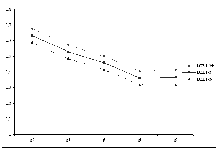
decline in the LOR[1x2] is highly significant and substantial (OR declines from
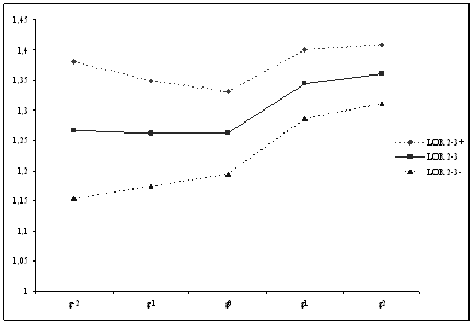
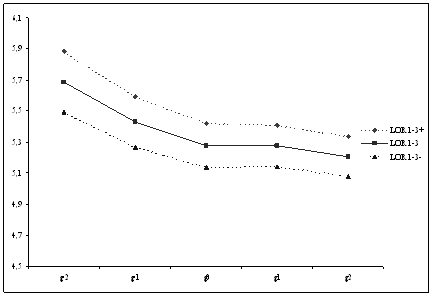
5,1 to 3,9 : -23%) ; LOR[1x3] face a significant decline and LOR[2x3] remain stable.
In this example, a loss of 23% of the OR is compatible with a realistic social
process of stable homogamy in a context of educational expansion. This result
is quite paradoxical.
 LOR[1x2] and 95% confidence interval from gen 1 to 5
 LOR[2x3] and 95% confidence interval from gen 1 to 5
LOR[1x3] and 95% confidence interval from gen 1 to 5

Here, the
correlation between the age at end of education of men and women remains unchanged
over generations, and the one change is an upward shift of the age at end of
education. However, the odds ratio diagnoses a significant and substantial
decline of the educational homogamy, supposedly net of marginal changes. The OR
as an accurate measure of homogamy in this context is quite problematic.
Discussion
For
purely categorical variables, the quality and precision of odds ratio as a
measure of the statistical link net of marginal changes are not contested.
However, when the real underlying process is based on numeric variables, the
use of odds ratios on categorized variables deriving from numeric ones could
give overestimated and may be fallacious results. A decline in the odds ratios
could be simply the result of a marginal change in the pertaining variable, and
not of a real change in the degree of association.
Hence,
the use of odds ratios without more effective verification on the underlying
marginal evolutions of the continuous process is problematic when we consider
education, for instance, but also for wage, income or wealth brackets, non
exclusively.
Anyway,
in social stratification, it is difficult to separate notions such as social
class/groups on the one hand and hierarchy which goes with quanta of educational/economic/social
resources on the ther. More systematic researches on the appropriateness of
odds ratios seem to be required to separate real results and artefacts.
Reference
Agresti A. 1984, Analysis
of Ordinal Categorical Data,